A Latticework of Inflation Models

Economists have repeatedly developed various theories for the origin of inflation and claimed that these theories were always valid everywhere. But history has shown that the theories – although they are useful - were only valid during certain time periods and under special circumstances. What is therefore needed is a system that assigns the various explanations of inflation to the specific circumstances for which they are particularly suited. This paper sets out such a system. Borrowing from Charlie Munger, I call it a “latticework of inflation models”.¹

In the first section I map the various inflation theories and then discuss and relate them to each other in the following sections. I find that during and after the pandemic several drivers of inflation were at work, so that several theories of inflation instead of just one allow a more comprehensive explanation of the inflation experienced during this period. The “latticework of inflation models” is also better suited than just one model for investigating the outlook for inflation.

Beware of the presumption of knowledge

Drawing on an earlier work², Friedrich August von Hayek criticized the trend in economic science towards emulating the physical sciences in his Nobel Prize lecture in 1974.³ He argued that economic systems have a much higher degree of complexity than natural systems, with the consequence that scientific methods applied in natural sciences are not applicable in social sciences, notably in economics. Disregarding the difference and applying methods used in natural science to economics can be seen as a category mistake, which leads to false conclusions. Economists tend to fall into this trap when they strife to “harden” their science and differentiate it from the “soft sciences” of the humanities. This behavior has been dubbed “physics envy”.⁴

Like other economists, scholars of inflation have repeatedly committed this category mistake as they developed various theories for the origins of inflation inspired by the circumstances prevailing at the time of their research and claimed that these theories were valid anytime and everywhere. Instead, these theories turned out to be valid only in certain historical and special circumstances.

The search for the ultimate theory

One of the oldest explanations of inflation is the quantity theory of money developed in the 16^th century. This theory, which has been attributed, among others, to the Prussian mathematician and astronomer Nicolas Copernicus (1473-1543) and the French political philosopher Jean Bodin (1530-1596), relates average prices in an economy to the amount of money in circulation.⁵ With the rise of Keynesian macroeconomics after World War II the quantity theory fell out of favor. The focus shifted to the real economy, in particular wages, as a source of inflation. In 1958, Bill Phillips, a New Zealand born economist working at the London School of Economics, discovered a relationship between unemployment and wage changes in UK data for 1861-1957.⁶ The step from there to a trade-off between unemployment and consumer price inflation was small.

The quantity theory made a comeback, when in the 1970s the trade-off implied by the Phillips-Curve collapsed and both unemployment and inflation rose. Excessive creation of money during the 1960s to fund the Johnson administration’s social policy of the “Great Society” and the Vietnam War had created an excess supply of US-Dollars, which drained the gold reserves of the US. In 1971 US President Richard Nixon therefore ended the peg of the US-Dollar to gold. The monetary overhang induced a depreciation of the exchange rate and created an inflation potential. When oil prices exploded due to the Yom Kippur War at the end of 1973, this potential was set free. Inflation increased, even though the economy weakened, and unemployment rose.

The new proponents of the old quantity theory – who called themselves “monetarists” - made from the simple quantity equation establishing a relationship between money, real GDP and prices a function with prices as the endogenous and real GDP, the velocity of money and the money stock as exogenous variables.⁷ By fitting this function to the data, they claimed to have created an instrument for central banks to steer inflation and dubbed it “monetary targeting”.⁸ This scheme worked for a while but collapsed when the function proved unstable and the money stock uncontrollable by the policy makers. This set the stage for the come-back of the Phillips-Curve.⁹

Central banks believed they could steer inflation by using the presumed stable and measurable relationship between unemployment and consumer price inflation. The new approach, dubbed inflation targeting, was supposed to avoid the pitfalls of monetary targeting and even allow central banks to smooth the business cycle. To this end, variations of unemployment were broken down in cyclical and structural components. Using “Okun’s Law”, the cyclical component was related to the aggregate capacity utilization of the economy, the so called “output gap”. During the 1990s, the approach seemed to work well, and the central banks even claimed credit to have created a “Great Moderation” of the business cycle.

During the first two decades of the 2000s, however, the strategy unraveled from two ends: First, deflationary pressures from the supply side (owing to technical progress and global trade integration) induced the central banks to set interest rates too low for balanced growth. The result were credit and asset price cycles instead of the previous business cycles. Second, again because of structural changes on the supply-side, the Phillips-Curve “flattened” and the relationship between wages and unemployment seemed to fall apart. As a result of their reliance on the Phillips-Curve, central banks incorrectly forecast low inflation during the pandemic and were surprised by its surge. Now, they are trying to regain control over inflation by making their policy actions “data dependent”. But this is just a euphemism for operating in theoretically unchartered territory and reacting ad hoc to new information.

Mapping the various inflation theories

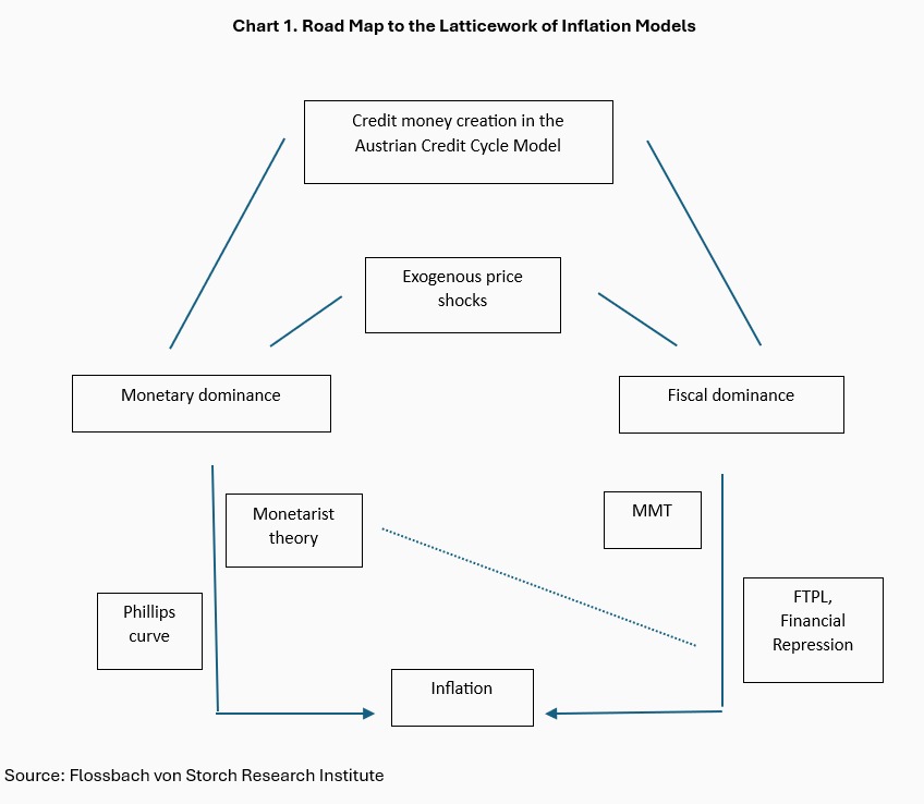
Without doubt, economists will busy themselves with developing the next “general theory” of inflation. For now, efforts focus on disentangling supply-side from demand-side drivers of inflation.¹⁰ By giving the supply-side drivers a prominent role, this research helps to exculpate the central banks for having missed the inflation surge. Sooner or later another “general theory” is likely to emerge from this. However, this will again be a futile effort as there is no inflation theory applicable always and everywhere like the theories in natural sciences. In the following, I therefore propose (hat tip to the late Charlie Munger) a “latticework of inflation models”, relating individual theories to specific applications and relating them to different economic regimes. Chart 1 gives the roadmap to the “latticework”. In the following sections, I discuss the various paths and junctions.

Credit money creation

Money matters. At least since the Roman Emperors mixed cheaper metals into the Denarius to fund government spending, this is a well-known fact. The silver content of the Roman coin fell from 95-98 percent in 267 BC to 5 percent by 274 AD.¹¹ Especially during the more rapid pace of debasement in the later years, price inflation became a problem. That money matters, was also well known to Chinese traders in the 9^th century AD who invented paper money as a substitute for unwieldy metal coins. When the state adopted this technique to fund expenses, it issued too many paper notes. As a result, China experienced hyperinflation in the era of the Yuan dynasty. Many years later, in the 15^th century during the Ming Dynasty, the emperor abolished the inflationary paper money and returned to silver coins.¹²

Money mattered, when gold came from South America to Europe on Spanish galleons in the 16^th century. The money stock and prices rose. As explained above, this lead Nicolas Copernicus and Jean Bodin to develop the quantity theory of money as an explanation for inflation. And when in the 17^th century paper money came from China to Europe, banks increased the money supply by covering only a fraction of the paper money issued against metal coins with the latter. Thus, the paper money supply could rise above the metal coin cover stock, leading to recurrent banking crises and inflation.¹³

All fetters were cut from money supply when US President Richard Nixon in 1971 ended the link of the US-Dollar to gold. From then on, money could truly be created “out of nothing”, namely simply through bank lending. The new money was aptly called “fiat money”, after God’s biblical word “let there be light”.¹⁴ Money production took place in a private-public partnership. Mostly private credit banks created money through lending while the (public) central bank steered the process by varying the rates on its loans to credit banks. The latter borrowed central bank money for use as collateral for inter-bank transfers of customer deposits and a substitute for inter-bank loans. As banks could not always rely on the availability of inter-bank loans and therefore had to allow for a possible recourse to loans from the central bank, the costs of central bank funding set a floor to banks’ lending rates.¹⁵

Although Ludwig von Mises had described money creation through bank lending and its potentially inflationary impact already in 1912, mainstream economics paid little attention to his insights and largely ignored the intricate process of money creation.¹⁶ As a result, mainstream economics assumed that changes in the money supply had no effect on real economic variables and proclaimed the “neutrality of money”. It ignored the point already made by Richard Cantillon, a 17^th century financial speculator and economist, that new money does not drop from heaven like rain but always enters the economy at a certain point, when it comes into the hands of specific economic agents who use it for specific purposes.¹⁷ Hence, an injection of new money affects some prices more than others and is not only associated with a loss of its purchasing power but also with a change in relative prices. This form of “non-neutrality of money” came to be known as “Cantillon-Effect”.

Newly created money can be spent or hoarded. In general, it will be spent when the share of money holdings in total wealth of an economic agent exceeds the desired level. What it will be spent for depends on the wealth composition of the agent who receives it. When new money is received by someone already holding the desired level of funds for purchases of consumer goods, it increases the share of money holdings relative to that of other assets above the desired level. Consequently, the economic agent will use the new money to purchase other assets, and the (money) price of these assets will increase until the desired portfolio structure is reestablished. In this case, new money creates “asset price inflation”. On the other hand, someone holding a lower level of consumption funds than desired will spend new money on the acquisition of goods. Consumer goods price inflation is the result.

Bank lending unaccompanied by increased government borrowing tends to stimulate asset price inflation. Banks lend against collateral when loan demand is stimulated by lower interest rates. Borrowers able to post collateral are wealthier than others and hence more likely to already possess the funds for their desired purchases of consumer goods. Hence, they may regard a decline in interest rates as an opportunity to buy more assets on credit. Asset prices increase because of both higher valuations due to lower interest rates and higher demand.

On the other hand, bank lending to the government for the funding of transfers to private households tends to raise consumer price inflation. Government transfers are often targeted to lower-income households with a deficit in funds for consumption. These households often have few assets and a high propensity to use new money for consumption. Hence, new money created for government transfers stimulates consumer demand and raises consumer prices.

Exogenous price shocks

Price increases of goods playing an important role in the economy, such as fuels, can have significant effects on other prices and the aggregate price level. These effects could only be neutralized if there were offsetting declines in other prices. This is next to impossible in the short term and often difficult even in the medium-term when production costs are sticky due to downward rigidities of wages. Moreover, offsetting price declines fail to materialize also in the long-term when the money supply is increased to accommodate a higher price level induced by the exogenous shock. A spiral of price increases
feeding on themselves could ensue, when the increase in the money supply is not restricted to a one-off event but renewed each time the price level has increased.

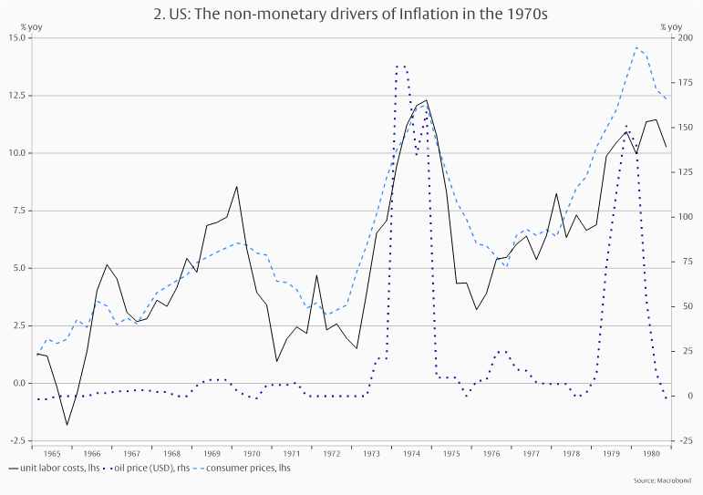
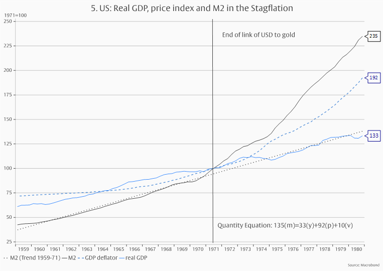
In the 1970s, the positive feed-back loop between increases of oil prices, wages and the money supply created engrained consumer price inflation (see Chart 2). Already during the 1960s the Federal Reserve allowed money supply growth to accelerate. Growth became even stronger after the Nixon administration in 1971 cut the peg of the Dollar to gold. Ample money supply turned into inflation when a surge in oil prices first raised other prices and then wages. Engrained inflation dampened economic growth because the distortion of relative prices induced by it created economic distortions and sapped economic efficiency. This toxic combination was dubbed “Stagflation”.

With the experience of the 1970s in mind, policy makers today are adamant about preventing “second round effects” of positive exogenous price shocks. At the same time, they find it too costly to suppress one-off increases in the measured price level. This approach requires a balancing act, allowing exogenous price shocks to work through the economy while preventing the emergence of second round effects. The act does not always succeed. Hence, exogenous price shocks are almost always associated with a temporary and sometimes with a longer-term increase in goods price inflation.

Monetary or fiscal dominance

When the government accepts a pure commodity money system, where the supply of money is given exogenously, or does not interfere with the central bank in the fiat credit money system, it submits its fiscal policy to the scarcity of money. The monetary policy of the central bank then “dominates” fiscal policy. In the opposite case, when the government relies on money creation as a means of financing its expenses, fiscal policy “dominates” the operations of the central bank associated with money creation.¹⁸

Different theories of inflation assume the one or the other regime, and their usefulness for explaining inflation depends on which regime exists. Since Roman times periods of monetary and fiscal dominance have alternated. Fiscal dominance emerges when the ability of a government to live within its means evaporates and new money is urgently needed to fund budget deficits. Monetary dominance takes over when the abuse of money creation by the government has debased the currency, boosted price inflation, and created enough dissatisfaction among the public to induce political change.¹⁹ In the following, I first discuss inflation theories applicable in the regime of monetary dominance and then move to theories suited to the regime of fiscal dominance.

Monetarist theory

As stated, the inflation during the 1970s brought back the quantity theory of money, which had been usurped after WWII by Keynesianism and the Philipps-Curve. In a talk in India in 1963, Milton Friedman proclaimed that “inflation was always and everywhere a monetary phenomenon”.²⁰ With this, he laid the ground for the monetarists’ believe that the central bank could control inflation when it controlled the money supply. They started out with the ancient quantity theory of money, encapsulated in the so-called quantity equation first introduced by Irving Fisher:²¹

P Y = v M,

where P denotes the price level, Y real gross domestic product (a proxy for real income), M the stock of money and v the so-called velocity of money, translating the stock variable M into a flow variable of money expenses v M, matching nominal GDP (or income). Next, they assumed that Y and v were determined by exogenous factors, such as the productive capacity of the economy and the longer-term trend in people’s desire to hold money units relative to units of nominal GDP, and solved for P. Thus, the price level becomes a function of the money stock:

Increases in the money stock raise the price level, decreases lower it. If the central bank can control the money stock, it can also control inflation.

The monetarists acknowledged that the central bank, while having full control over its own liabilities in the form of the central bank money stock, has only indirect control over the liability of banks in the form of money deposits. But they thought that the “money multiplier”, the ratio of total money to central bank money, moves only little, or that its movements can be modeled.²² To reflect the lack of full control of the central bank of the money stock, they established money growth as an “intermediate” target for the central bank for reaching the “final” target, the price level - and dubbed this approach to monetary policy “monetary targeting”.²³

The quantity equation is an identity, and it is a tautology to say that big moves of M influence P when they are not offset by moves of Y or v. History has many examples where M dominated all other influences on P. However, it goes too far to say that moves of M always impact P, because offsets can and have occurred. Moreover, there may be entirely different factors affecting the price level that are not captured by the quantity equation (remember exogenous price shocks). Hence, the claim of the monetarists to have a comprehensive explanation of inflation is overdone.

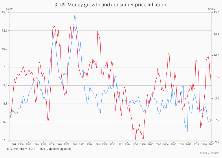
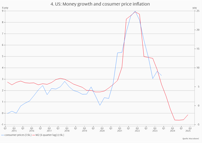
Milton Friedman warned that the lags of money growth on inflation are long and variable.²⁴ History certainly bears this out. As Chart 3 shows, money growth affected consumer price inflation in the 1970s with a three-year delay. In the more recent episode of 2020-22, the lag fell to one year and a half (Chart 4). But increases of money growth not always preceded increases in inflation. As can be seen from Chart 3, both variables moved in opposite directions in the mid-1980s and the mid-1990s. Moreover, there was no clear correlation through most of the 2000s, except in 2020-22.

Expositions as in Charts 3-4 suffer from the shortcoming that they compare a stock variable, the money aggregate, to a variable – prices – associated with a flow – goods consumed during a certain period. But a high stock of money can fuel demand and hence consumer price inflation over a considerable period of time, until it is fully absorbed in aggregate demand and prices. This is illustrated in Chart 5, where US real GDP, the money stock M2, and the GDP deflator are plotted.

Until the early 1970s, money, real GDP, and prices moved along stable trends, with the trend of the money stock slightly steeper than that of real GDP and the deflator due to a trend decline in money velocity (reflecting a desire for the holding of more money balances over time). This changed after the peg of the US Dollar to gold was cut in August 1971 - and the money order moved from a gold-backed fractional reserve holding system to the fiat-credit-money system of today. The money stock and prices rose on a steeper trend while real GDP continued at roughly the same trend as before. The quantity equation can be used to attribute the increase in the money stock until the 1980s to increases in real GDP (y), prices (p) and a decrease in velocity (v, see Chart 5). With real GDP and velocity changing only little, the bulk of the rise in the money stock was absorbed by the increase in prices.

Moreover, the assumption that central banks can control money creation ignores the fact that in the fiat credit money system it is commercial banks that create money through credit extension, and that commercial banks have considerable leeway in defining what money is. The idea of monetary targeting becomes untenable when the central bank can neither clearly define the target (because the banks invent new forms of “money”) nor has the means to reach it (because it cannot control the money generation of banks strictly enough). Thus, the idea that there is a causal and stable relationship between changes in the money supply and the price level, and that the central bank can use this relationship to control inflation is untenable.

Money supply may be the most important source of inflation under certain circumstances, but it may not matter at all under other circumstances. Claudio Borio and his co-authors find the strength of the link between money growth and inflation depends on the inflation regime: it is one-to-one when inflation is high and virtually non-existent when it is low.²⁵ Consequently, cross section analyses including countries with different inflation regimes or time series analyses for individual countries experiencing different inflation regimes over a long period find a strong link between money growth and inflation.

The Phillips-Curve

When money takes a backseat in the generation of inflation – which is mostly the case when both monetary and fiscal policies are executed with moderation – developments in the real economy may become the key driver of price developments. Explanations of inflation under these circumstances are inspired by the simple idea (imported from microeconomics) that temporary imbalances between supply and demand trigger price changes to restore balance.

Obviously, it requires imbalances in a market that affects all other markets to move all prices. As already mentioned, it was Alban William Housego (“Bill”) Phillips who in an empirical study published in 1958 put the labor market in the center of inflation theory. Looking at changes in wages and unemployment rates he found that the two variables moved inversely. When unemployment was high, wages declined, and when it was low, they increased. This insight prompted a myriad of further investigations, both empirical and theoretical, which culminated in the thesis that inflation is a function of the output gap, i.e., the difference between actual and potential GDP. A positive difference, i.e., actual GDP greater than its potential, induces inflation above longer-term inflation expectations, a negative difference pushes inflation below this level.

The simple output gap-inflation model has been upgraded technically to ever more sophisticated levels and has been integrated into the New Keynesian Dynamic Stochastic General Equilibrium Models cherished by the inflation forecasters of central banks. However, the economic engineering has neither overcome the basic flaws of the model exposed by many economists nor improved the accuracy of the inflation forecasts derived from it.²⁶ Apart from its many limitations discussed in the economic literature it suffers from two basic shortcomings.

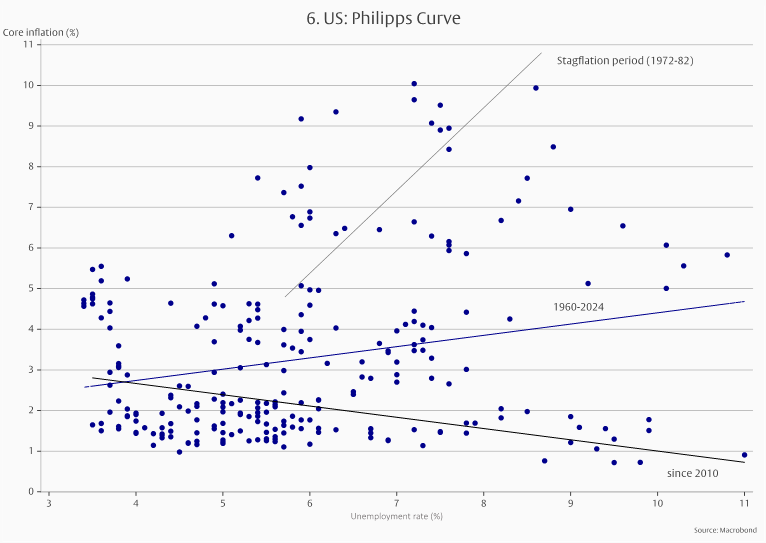
First, the Phillips-Curve is unstable over time. Sometimes it holds, sometimes the negative correlation between unemployment and wage growth breaks down. This is illustrated in Chart 6. There was a moderately positive but statistically insignificant correlation between the unemployment rate and core consumer price inflation in the US in 1960-2024. During the “stagflationary” 1970s, the slope was even more strongly positive. A negative slope of the curve, as it should be, emerged in the period since 2010, but the explanatory power of the equation is relatively poor (with an adjusted R² of 0.19).

Second, the Phillips Curve excludes other important drivers of inflation beyond supply-demand imbalances in the real economy, whose alternating appearance and disappearance may well explain the instability of the curve. Using spectral analysis, Brian Reinbold and Yi Wen find that in the very short run, there is no systemic relationship between inflation and unemployment; in the intermediate run, which includes the business cycle frequency, they are strongly negatively correlated (as they should be); and in the very long run the Phillips curve is strongly positively sloped.²⁷

Modern Monetary Theory

We now move from monetary to fiscal dominance and start in this regime with a theory that puts fiscal policy explicitly in charge of controlling inflation. The so-called “Modern Monetary Theory” (MMT) has been stated in normative terms and can be seen as the ultimate framework for fiscal dominance.²⁸ But the “theory” has its roots in positive experience with monetary financing of government expenses. Thus, it is neither modern nor a theory, but certainly “monetary”.

At its core is the historical experience that inflation rises when a government increases the supply of its sovereign money to purchase goods and services. The debasement of the currency by subsequent Roman emperors may not have been the first application of this leg of MMT, but certainly a prominent one, followed by many more in the following two millennia. However, while creating inflation through monetary financing of government spending has always been successful, the reverse has rarely worked. The reason is not that there were asymmetric effects associated with more and less government spending, but that politicians are unable to use fiscal belt tightening as a tool for fighting inflation.

“A dog is more likely to stock up on sausages than a democratic government is to build up a budget reserve”, the great economist Joseph Schumpeter already remarked. Had the proponents of MMT be a little better read, they would not have committed the beginner’s mistake of ignoring this wisdom. Yet, this does not invalidate the observation from historical experience that a government merrily debasing its sovereign currency is a powerful driver of inflation of prices expressed in this currency. Thus, MMT provides a useful explanation of the role of government and money creation for inflation but is too naïve about politics to offer a normative framework for a combined fiscal and monetary policy.

Fiscal Theory of the Price Level

A positive theory of inflation giving fiscal policy center stage is the “fiscal theory of the price level” (FTPL).²⁹ Like MMT, FTPL takes a “Chartalist” view of money. For Georg Friedrich Knapp, the originator of “Chartalism”, money was a creation of the state by legislation, and not, like for Adam Smith, a means of transaction elected by people through consensus. Money creation by the state opens the possibility of its use as a funding instrument for the state. What the state has created and declared “legal tender”, it can use to acquire goods and services from its citizens. Thus, FTPL regards money simply as another instrument for financing government expenditures.

While MMT looks at flows only (in the form of changes in the money stock and the difference between government spending and revenue), FTPL widens the view to stocks. In particular, it regards the balance sheet identity as the key constraint to the funding of government assets. All government liabilities need to be covered by the present value of all future budgetary surpluses in real terms.³⁰ Thus,

where M, B, and P on the left-hand side of the equation denote money, bonds, and prices. On the right-hand side of the equation, E is an expectations indicator, S budgetary surpluses in price-adjusted terms, ß a time discount factor, and t a time indicator.

An increase in the expected value of future real budget surpluses can be funded by new issues of bonds, money or both without affecting the price level. If, however, the government issues more debt (in the form of money and/or bonds) and the present value of expected future real budget surpluses does not increase – because, for instance, the public does not fulfill David Ricardo’s equivalence theorem and hence does not expect tax hikes in the future – balance sheet identity is restored by an increase in P. On the other hand, if the government reduces debt without an impact on expected future budget surpluses, the price level falls. Thus, government borrowing can have a direct impact on inflation. If the funding instrument is money, FTPL stipulates a relationship between fiscal policy and inflation identical to that proclaimed by MMT.

The key difference between FTPL and MMT is that the former assumes fiscal policy to be motivated by other objectives than the desire to influence inflation while the latter regards fiscal policy as motived primarily by the government’s desire to achieve a certain inflation objective. In FTPL, the balance sheet identity establishes the constraint for a fiscal policy consistent with price stability. In MMT, such a constraint is unnecessary, because the supreme objective of fiscal policy is price stability. And changes in prices are explained by temporary imbalances between aggregate supply and demand, caused by fiscal policy financed by money issuance.

While MMT takes a rather traditional Keynesian view of the generation of inflation, it makes an extremely narrow and unrealistic assumption about the objectives of fiscal policy. But if fiscal policy has other objectives which it puts above price stability, the first leg of MMT, the generation of inflation, always works, while the second leg, the reduction of inflation, almost never works. By contrast, FTPL takes a much more realistic view of the objectives of fiscal policy but is not entirely clear about way the balance sheet identity connects fiscal policy with the price level.

In the above equation, adapted from John Cochrane (op. cit.), changes in expectations of future real budget surpluses lead to changes of the price level when nominal liabilities are unchanged. However, it is difficult to imagine that people would spend less when they expect future government surpluses to increase, so that the price level falls, and real liabilities increase to match expected surpluses. Similarly, would they spend more, if expected surpluses decline, to raises the price level and reduce the real value of liabilities? They would have to hold rational expectations and act in line with David Ricardo’s “equivalence” theorem. But it is more likely that people do not hold rational expectations and are myopic regarding future taxation.

A more realistic view of fiscal policy affecting the price level would see the left-hand side of the above equation, government debt, drive inflation. Increases in government debt through issues of money or securities, which are not offset by increases in expected future budget surpluses, raise the price level in any event. Assume that a government issues more debt to fund expenses without taking action to ensure a matching increase in expected future budget surpluses. In this case, rising interest rates can soon be expected to lead to unsustainable levels of interest expenses. The government will induce the central bank to manipulate nominal interest rates below the rate of inflation to ease the debt service burden. A negative real interest rate resulting from this manipulation induces more consumption and less saving. Excess demand for goods and services then raises the price level to realign real government liabilities with expected real budget surpluses. Empirical studies have found support for this mechanism, which has been dubbed “financial repression”.³¹

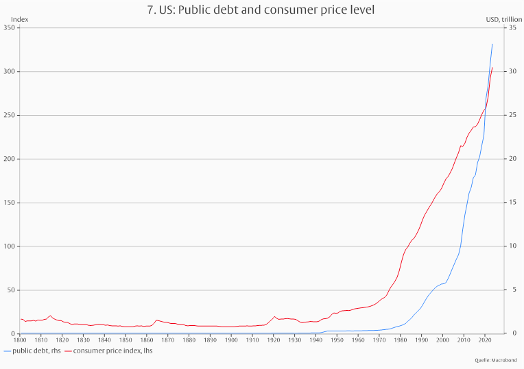
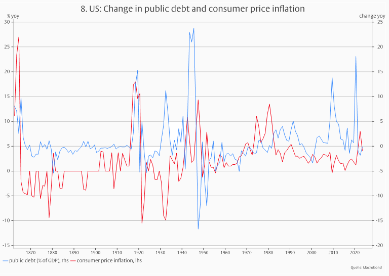
As Chart 7 shows, public debt and the consumer price level in the US have moved in tandem with each other since 1800. However, other variables may have been responsible for the long-term positive correlation. Hence, it is worth comparing consumer price inflation and changes in public debt, although the theory is explicitly stated in levels. As Chart 8 shows, there is no clear correlation over the entire sample period, but when government borrowing surges in periods of extreme stress, like in the two world wars of the 20^th century and the pandemic of 2020-22, surges in public debt are associated with or precede increases in consumer price inflation. This suggests that the Fiscal Theory of the Price Level may have a good explanatory power in periods of serious fiscal stress. John Cochrane explains this in the following way: “If the government runs a big deficit, but people trust that the deficit will be repaid by higher subsequent surpluses, then people are happy to hold the extra debt rather than try to spend it, and there is no inflation… Fiscal theory only predicts inflation when debt is larger than what people think the government will repay”.³²

Outlook and conclusion

In this paper I argued that it is mistaken to assume, a general theory can be found to explain inflation though all times and in any circumstances. Instead, it is more useful to identify the explanatory power of various inflation explanations in different time periods and under different circumstances. The time of the Coronavirus Pandemic, when inflation was driven by various factors in short time sequence, provides a particularly useful period for the study of various drivers and their relevance.

During the early phases of the pandemic, all drivers were active. Delivery chains broke and prices of inputs and commodities surged. The war in Ukraine added to commodity price pressures. Activity was “locked down” and supply plunged. At the same time, governments compensated companies and workers for lost earnings. Central banks provided the financing through money printing as tapping the capital markets would have raised interest rates. Thus, excess money supply led to excess demand. As inflation took off workers demanded higher wages to compensate for the loss in purchasing power, adding another cost push.

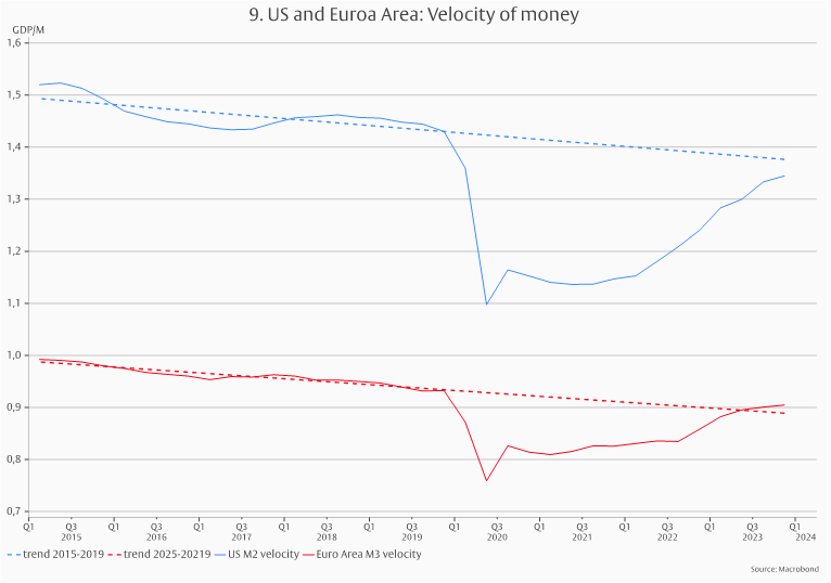
When central banks belatedly began to reverse their extremely expansionary monetary policy, the money stock stopped growing. At the same time, high inflation eroded the purchasing power of excess money balances. As a result, money velocity (the ratio of GDP to the money stock) returned to more normal levels. At the beginning of 2024, it seemed that excess money balances had ceased to contribute to inflation in the euro area and had been reduced to a small size (if any) in the US (Chart 9).

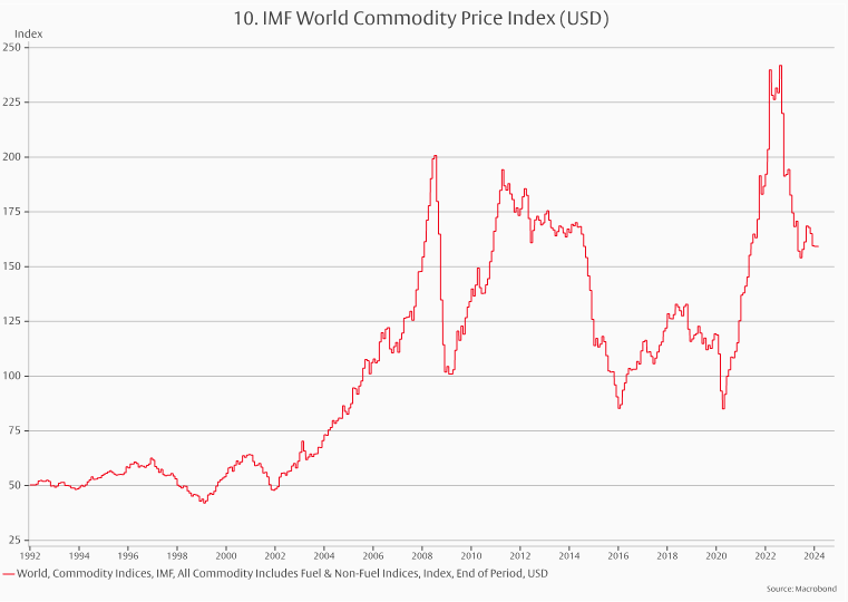
At the same time, delivery chains were gradually restored, and commodity supplies adjusted to the embargo imposed by western countries against Russia. Consequently, commodity prices fell from their earlier highs (but remained above pre-pandemic levels, Chart 10).

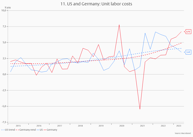
While the monetary and exogenous drivers of inflation abated, wage growth continued to exert upward pressure on inflation. With productivity growth in the euro area much lower than in the US, unit labor cost growth accelerated sharply in the euro zone but eased somewhat in the US. Nevertheless, also in the US unit labor cost growth remained above the level consistent with 2 percent inflation at the beginning of 2024 (Chart 11).

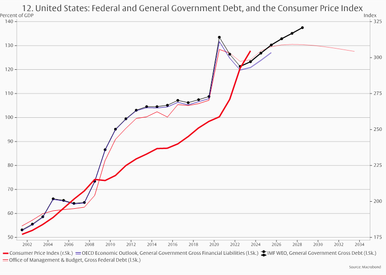
Moreover, “re-shoring” of activities to reduce delivery risks and geo-economic fragmentation are likely to exert upward pressure on prices for some time to come. And the Fiscal Theory of the Price Level suggests that growing government debt will induce continuous inflation pressures to maintain equality between real assets and liabilities in governments’ balance sheets (Chart 12). Thus, the key question for the outlook for inflation is whether FTPL holds or not. If it does, we should expect elevated inflation and low or negative real interest rates in the future. Under these circumstances, real assets should give higher returns than nominal assets.

¹ Charles T. Munger, Poor Charlie’s Almanack. 2005.

² Friedrich August von Hayek, The Counter-Revolution of Science: Studies on the Abuse of Reason, first published in 1952.

³https://www.nobelprize.org/prizes/economic-sciences/1974/hayek/lecture/

⁴ See, for instance, Philip Mirowski, More heat than light: Economics as Social Physics, Physics as Nature’s Economics. Cambridge University Press (New York) 1989.

⁵ See J. Taylor: Copernicus on the Evils of Inflation and the Establishment of a Sound Currency. In: Journal of the History of Ideas. 16 (1955), p 544: „Money loses its value when it is issued in too great a quantity.“ And D. P. O'Brien, "Bodin's Analysis of Inflation." History of Political Economy, Duke University Press Volume 32, Number 2, Summer 2000, pp. 267-292

⁶ A.W. Phillips, "The Relationship between Unemployment and the Rate of Change of Money Wages in the United Kingdom 1861-1957". Economica. 25 (100) 1958, pp. 283–299.

⁷ A basic work laying the foundations to monetarism is Milton Friedman and Anna Schwartz, A Monetary History of the United States, 1867–1960. Princeton University Press 1963.

⁸ See, for instance, Karl-Heinz Tödter, “Monetary Indicators and Policy Rules in the P-star Model”, Discussion Paper 18/02, Deutsche Bundesbank June 2002.

⁹ See Frederic S. Mishkin, “From Monetary Targeting to Inflation Targeting: Lessons from the Industrialized Countries”. Graduate School of Business, Columbia University and National Bureau of Economic Research, January 2000.

¹⁰ See, for instance, Marta Bańbura, Elena Bobeica, and Catalina Martínez Hernández, “What drives core inflation? The role of supply shocks.” ECB Working Paper No 2875, 2023.

¹¹ See, for instance, William Goetzmann, Money Changes Everything. Princeton University Press 2016, Chapter 7, and “The Great Denarius Debasement”, Gold Avenue, 31 July 2020 (https://www.goldavenue.com/en/blog/newsletter-precious-metals-spotlight/the-great-denarius-debasement).

¹² Goetzmann (op.cit.), Chapters 8-9.

¹³ See Thomas Mayer, Das Inflationsgespenst. ECOWIN (Salzburg) 2022.

¹⁴ The term “fiat money” had of course already existed before 1971. The evolution of the term and its adoption into economic language was a gradual process influenced by the development of monetary systems over centuries. The term became more commonly used among economists and in financial literature during the 19th and 20th centuries as nations increasingly moved away from commodity-based currencies (like the gold standard) to fiat currencies.

¹⁵ See, for instance, Thomas Mayer, Austrian Economics, Money and Finance. Routledge (Milton Park and New York) 2018 for a more detailed exposition.

¹⁶ Ludwig von Mises, Theorie des Geldes und der Umlaufsmittel. Duncker & Humblot (München und Leipzig) 1912.

¹⁷ Ricard Cantillon, Essai sur la Nature du Commerce en Général. Paris 1755.

¹⁸ Fiscal dominance can be explicit, when the government takes over the control of the money printing press, or implicit, when reckless bond issuance by the government forces the central bank to prevent the government’s bankruptcy by printing money. See Thomas J. Sargent and Neill Wallace, Some Unpleasant Monetarist Arithmetic, Federal Reserve Bank of Minneapolis Quarterly Review Vol. 5, N0. 3 (1981).

¹⁹ See, for instance, monetary reform to end hyperinflation in the German Reich in 1923.

²⁰ See https://www.hoover.org/research/inflation-true-and-false#:~:text=%E2%80%9CInflation%20is%20always%20and%20everywhere,gave%20in%20India%20in%201963 and Milton Friedman, Inflation, Causes and Consequences, Asian Publishing House 1963.

²¹ Irving Fisher, The Purchasing Power of Money. The Macmillan Co. (New York) 1911.

²² See Karl Brunner. A schema for the supply theory of money. International Economic Review, 2(1), 1961, pp. 79-109, and Karl Brunner and Allan H. Meltzer. The place of financial intermediaries in the transmission of monetary policy. American Economic Review, 53(2), 1963, pp.: 372-382.

²³ See OECD, Monetary Targets and Inflation Control, Monetary Studies Series, OECD 1979.

²⁴ Milton Friedman and Anna Jacobson Schwartz (op.cit.).

²⁵ Claudio Borio, Boris Hofmann and Egon Zakrajšek, “Does money growth help explain the recent inflation surge?” BIS Bulletin No. 67, 26 January 2023, and Luca Benati, “Long Run Evidence on Money Growth and Inflation”, ECB Working Paper Series No. 1027 (March 2009).

²⁶ See, for instance, Daniel Gros and Farzaneh Shamsfakr, The ECB’s normalisation path. Center for European Policy Studies (Brussels) 20 June 2022.

²⁷ Brian Reinbold and Yi Wen, “Is the Phillips Curve Still Alive?”, Federal Reserve Bank of St. Louis Review, Second Quarter 2020.

²⁸ See Rodger Malcolm Mitchell, Free Money: Plan for Prosperity. PGM International ,1 September 2005.

²⁹ See Eric M. Leeper, "Equilibria under 'Active' and 'Passive' Monetary and Fiscal Policies". Journal of Monetary Economics. 27 (1) 1991, pp. 129−147.

³⁰ See John H. Cochrane, The Fiscal Theory of the Price Level. Princeton University Press 2023.

³¹ See, e.g., Carmen Reinhardt and M. Belen Sbrancia, “The Liquidation of Government Debt,”. NBER Working Paper 16893, March 2011.

³² John H. Cochrane, “Fiscal histories”, Journal of Economic Perspectives, 36(4), 2022, p. 127

Legal notice

The information contained and opinions expressed in this document reflect the views of the author at the time of publication and are subject to change without prior notice. Forward-looking statements reflect the judgement and future expectations of the author. The opinions and expectations found in this document may differ from estimations found in other documents of Flossbach von Storch AG. The above information is provided for informational purposes only and without any obligation, whether contractual or otherwise. This document does not constitute an offer to sell, purchase or subscribe to securities or other assets. The information and estimates contained herein do not constitute investment advice or any other form of recommendation. All information has been compiled with care. However, no guarantee is given as to the accuracy and completeness of information and no liability is accepted. Past performance is not a reliable indicator of future performance. All authorial rights and other rights, titles and claims (including copyrights, brands, patents, intellectual property rights and other rights) to, for and from all the information in this publication are subject, without restriction, to the applicable provisions and property rights of the registered owners. You do not acquire any rights to the contents. Copyright for contents created and published by Flossbach von Storch AG remains solely with Flossbach von Storch AG. Such content may not be reproduced or used in full or in part without the written approval of Flossbach von Storch AG.

Reprinting or making the content publicly available – in particular by including it in third-party websites – together with reproduction on data storage devices of any kind requires the prior written consent of Flossbach von Storch AG.

© 2024 Flossbach von Storch. All rights reserved.