07.08.2023 - Studies
The yield curve serves as an early indicator of recessions. Since 1970, inversions of the US-yield curve have always been followed by a recession. But can we rely upon this relation in the future as well? And can this interest rate signal be used for equity investments? Our research shows that the yield curve has sent useful signals for both economic forecasting and equity investing. Whether this will hold true for the future is a question that remains open (as always).
A yield curve shows the yield of bonds with the same quality for different maturities. Typically, yields on longer-maturity bonds are higher than those on shorter maturities because investors (with an investment horizon to final maturity) demand a "waiting premium." An inverted curve means that the yields of short-term bonds are higher than those of long-term bonds. This is only the case if investors expect a future decline in short-term interest rates controlled by the central bank because of a looming recession.
In the war and post-war period, the economy did not play a significant role in interest rate formation because other influences were stronger. From 1942 onward, the U.S. Federal Reserve fixed the interest rates on short-term bonds (Treasury Bills) at a very low level to finance the war. Interest rates on long-term bonds (Treasury Notes) were capped but were always higher than the fixed Bills. Although explicit control of the yield curve ended in 1951, the Fed continued to buy Treasury Bills to facilitate government financing, making inversion of the yield curve almost impossible.
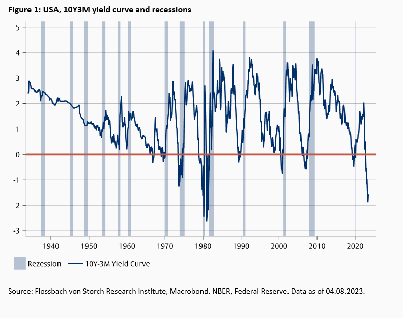
From the 1970s onward, the relationship changed. Now, the business cycle played a major role and a curve inversion was always followed by a recession (Fig. 1). Since the 1970s, the inversion of the yield curve was mostly caused by the Fed raising its key interest rate in response to rising inflation or inflation expectations. Because markets assumed that fighting inflation would require a recession in which policy rates would fall again, long-term rates generally rose less and the curve inverted. One exception was 2020, when the economy fell into recession due to the pandemic without any policy rate hikes.
The probability of a recession can be estimated from the signals of the yield curve. The standard method is a probit model.1 Among the many possible variations, we opt for a simple specification with the yield curve and the fed funds rate as explanatory variables, as shown in equation (1).

The variable NBERt equals 1, if the National Bureau of Economic Research (NBER) has dated a recession for month t. We search for the optimal forecast horizon by incrementally (i.e., month by month) increasing the variable h in repeated estimates. On the right side are the term spread (SPREADt10Y-3M), i.e. the difference between the yields on 10-year and 3-month government bonds, the fed funds rate (FFt) and an interaction term between the term spread and the fed funds rate. The reason for the interaction term is that the signal from the yield curve can vary in strength depending on the level of the policy rate (Cooper et al. 2020). The function Φ(⋅) is the distribution function of a standard normal distribution. The data are available from 1953.
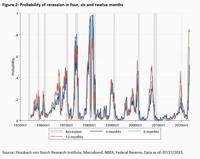
Because the time lag between a curve inversion and the beginning of a recession was different in each episode, the model calculates different recession probabilities depending on the forecast horizon of h months. Therefore, we first estimate twelve models, each with a forecast horizon of h = 1, ..., 12. As an illustration of the estimation results, we use here the estimated recession probabilities in four, six and twelve months (Fig. 2). The recession probabilities rise sharply ahead of the recessions beginning in the 1970s, when the Fed raised short-term interest rates, first hesitantly and later drastically, to combat inflation. The recession signals from the model later weaken again, but with the current curve inversion are almost as high as in the 1980s.
These estimates show that the yield curve and the fed funds rate correlated with recession episodes with some lead. However, they only look into the past and say little about the model's ability to forecast the future.
We now extend the analysis to estimate the model's forecasting ability into the future. To this end, we calculate the probability of a recession starting in January 1985 in subsequent months using data available only up to this forecast period. Thus, the fed funds rate and the yield curve are initially available for the model only up to January 1985. For February 1985, we estimate the model again using the new available data, and so on. These estimates are renewed-and the coefficients thus "updated"-until the yield curve inverts. From the following month onward, the model remains unchanged because, as the curve begins to invert, there is uncertainty about the occurrence of a recession. Using the coefficients unchanged since the last estimate, we now continue to calculate the recession probability month by month with the new data on the yield curve and fed funds rate.
Only when the full dating of the recession is published we start updating the model again with new coefficient estimates. The NBER dates the beginning and end of recessions with a significant time lag. For example, according to the NBER's dating, the Great Financial Crisis began in December 2007 and ended in June 2009. However, the beginning of the recession was not announced until December 2008 and the end until September 2010. Thus, there was no clarity about the recession dating during the financial crisis. Therefore, for the purpose of estimating the recession probabilities in each case, we assume that only the dating of past recessions was known.
Another parameter that must be reselected when the curve inverts is the forecast time window h. When the curve starts to invert, we estimate - as in the previous section - twelve models each with a forecast horizon of h = 1, ..., 12 months. From each of these estimates, we select the forecast window h that indicated the highest recession probability before the last recession. This results in a forecast time window of six months for the curve inversions before 1990 and a window of eight months for the later curve inversions.
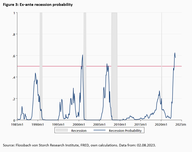
According to this real-time application of the method simulated for the past, ex-ante probabilities for the recessions from 2000 onwards are over 50% (fig 4.). For the (fairly mild) recession of 1990, however, the signal was less than 50%, while today the probability is as high as before the burst of the dotcom bubble.
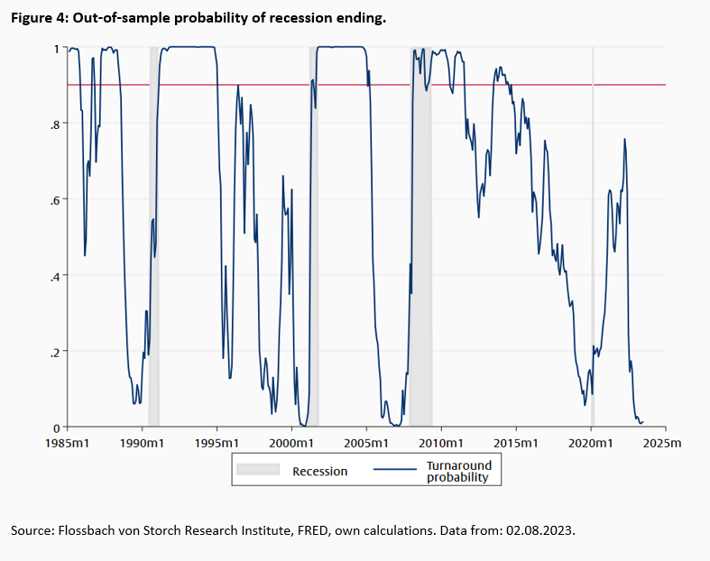
In the next step, we define a new model to estimate the probabilities of the end of a recession. As in equation (1), the second model is a probit model with the yield curve and the fed funds rate as explanatory variables. On the left-hand side of the equation, we set the endogenous variable to zero during a recession and to one in the twelve months following. We disregard data outside these periods because then the question of the end of a recession is not relevant. Since the NBER defines a recession as the period from the peak to the trough of the business cycle, a new upswing begins at its observed end.
The model for the end of the recession, like that for the beginning, is estimated recursively month by month, starting when the yield curve is inverted. The estimates are used to calculate the turnaround probabilities (Fig. 4). The end of all recessions, with the exception of the pandemic recession, was correctly predicted before the actual end, but with different forecast horizons.
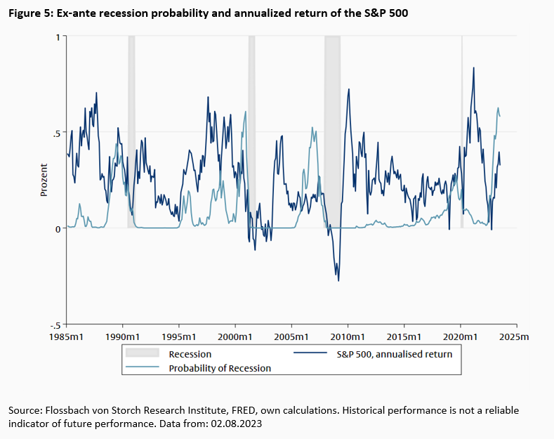
It has become clear from the estimation of recession probabilities that the yield curve and the fed funds rate can provide helpful signals for the business cycle. The lag between the recession signal and the recession start, and the recovery signal and the recession end, however, are different in each episode. Therefore, investors may get a little more information about the onset of a recession from the estimates, but must continue to maneuver in an uncertain environment. This raises the question of whether investors in equities could hedge against a recession if it has a strong impact on equity prices (as seen in Fig. 5).
It is possible to hedge a stock portfolio by purchasing put options. If the share price falls below the strike price of the option, the option hedges the further decline. However, if the share price does not fall below this value during the term of the option, the buyer loses the premium paid for the insurance.
The Chicago Board of Options Exchange has published a Put Protection Index (PPUT) since July 1986. This index tracks the performance of a hypothetical investment strategy involving the purchase of the S&P 500 Index and the simultaneous purchase of put options on the S&P 500 Index. Monthly put options are purchased with a strike price 5% below the current price. Because we are not aware of any index fund that tracks the PPUT index, our analysis is based on the hypothetical PPUT portfolio of the CBOE.2
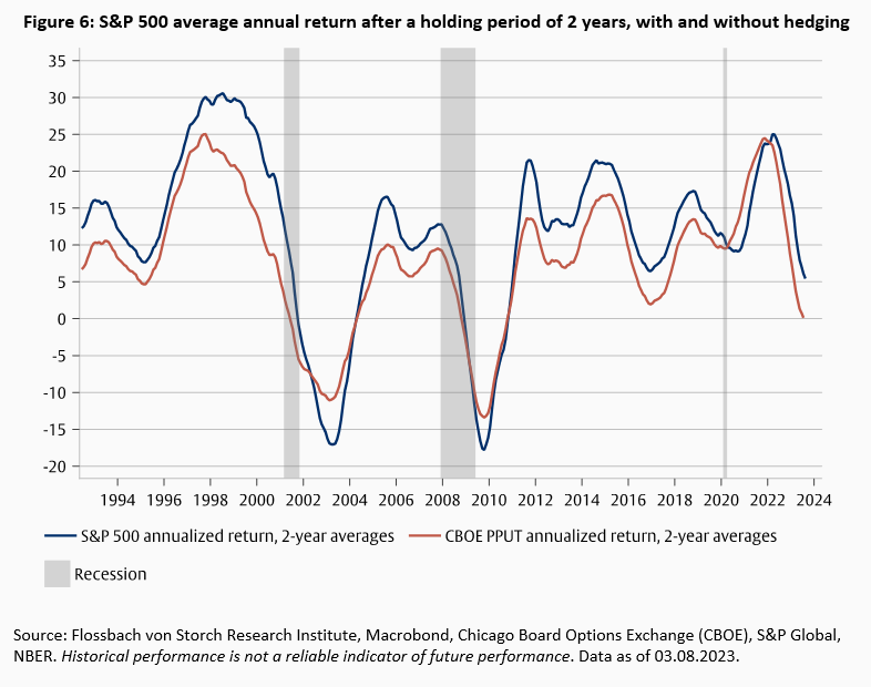
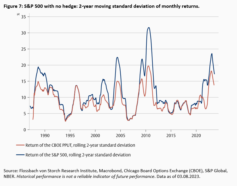
A fully hedged PPUT portfolio has generated an average annualized return of 7.4% since June 1986, compared with an 8.1% annual return for the unhedged S&P 500 over the same period. For a rolling holding period of two years, the average annualized return of the hedged portfolio was slightly higher than that of the unhedged portfolio after the bursting of the dotcom bubble , after the Great Financial Crisis, and after the Covid pandemic (Fig. 6). Elsewhere it was lower due to the hedging costs. The volatility of the hedged portfolio has been lower than that of the unhedged portfolio over the entire period. But the moderate reduction comes at the cost of a yield loss, which creates a considerable shortfall over time.
Thus, throughout hedging is associated with a loss of returns that is unlikely to be offset by the moderate reduction in portfolio volatility. But what if the hedge is only intermittent based on the estimated recession probabilities? To do this, assume that the put option is purchased when the ex ante recession probability exceeds 50%. The hedge is unwound when the recovery probability exceeds 90%.
Under this strategy, the total return of the "Recession Hedged" portfolio is slightly higher than the unhedged portfolio (Fig. 8). The total return would have been slightly better if the model had flagged the 1990 and 2020 recessions. Moreover, the forecasts of recession starts are as crucial as those of recession ends. Had we exited the hedging strategy a few months earlier in the 2001 and 2008 recessions, the total return would have been lower than the return of the unhedged portfolio.
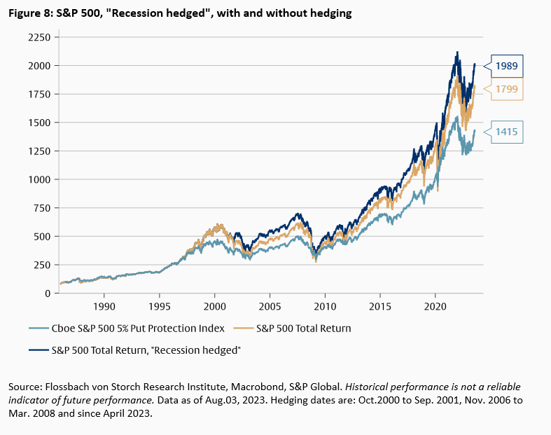
The hedging strategy generated an average annual return of 8.4% to date, 0.30 percentage points higher than the unhedged S&P 500 portfolio and one percentage point higher than the fully hedged portfolio (Table 1). Volatility after the hedging strategy is slightly lower than that of the S&P 500 but significantly higher than that of the end-to-end hedged portfolio. These results suggest that a strategy that takes into account the recession signals in the yield curve may be able to generate excess returns with slightly reduced volatility.
Table 1: Average annual returns and volatility ( July 1, 1986 to August 3, 2023)
| Average annual return | Annualized volatility | |
| S&P 500 | 8.10 % | 18.57 % |
| Hedging strategy | 8.40 % | 18.32 % |
| PPUT Index | 7.40 % | 13.59 % |
Source: Flossbach von Storch Research Institute, Macrobond, own calculations.
The success of the hedging strategy depends on the accuracy of the recession signals. As with any model, the forecasts are based on the regularities that can be inferred from the past. Each time, however, things could turn out differently. The model would have missed the recessions of 1990 and 2020. For the current economic development, on the other hand, there is a risk of a false forecast of the start of the recession.
The model shows a recession probability of over 90% since April 2023. For our hypothetical hedging strategy, this means that since April the premiums for put options have been paid. If instead of the predicted recession the economy "soft lands", the hedging costs would be lost.
In the long term, practical implementation would have to take into account that premiums for put options would rise if the hedging strategy became popular. This could erode the additional return. In addition, for more complex portfolios than the S&P500 portfolio studied here, the basis risk in hedging is likely to increase and also reduce the attractiveness of the potential excess return.
The yield curve is considered a good indicator for recessions. Since 1970, inversions of the curve in the US have always followed a recession. Using a simple early warning system, we have shown that the start of recessions in the US economy could have been predicted ex-ante using the yield curve. A hedging strategy for an equity portfolio based on these forecasts using put options could have improved performance.
But our model failed to see two of the last four recessions coming because the signals from the yield curve were not strong enough in advance. Would we have continued to pursue the hedging strategy based on the model after these mispredictions? And should we trust the current forecast of a recession with a certainty of over 90% based on probability theory, when in reality there is "radical uncertainty" that cannot be calculated?3 Ultimately, the crucial question is whether the recession model and the link between the U.S. economy and the stock market remain structurally stable over time. Unfortunately, our analysis cannot provide answers to these questions.
Borio, C. E., Drehmann, M., & Xia, F. D. (2018). The financial cycle and recession risk. BIS Quarterly Review December.
Cooper, D., Fuhrer, J. C., & Olivei, G. (2020). Predicting recessions using the yield curve: The role of the stance of monetary policy. Federal Reserve Bank of Boston Research Paper Series Current Policy Perspectives Paper, (87522).
Wright, J. (2006). The yield curve and predicting recessions (No. 2006-07). Board of Governors of the Federal Reserve System (US).
1 See for example Wright (2006), Borio et al. (2018) und Cooper et al. (2020).
2 An alternative approach would be to combine an S&P500 ETF with an inverse S&P 500 ETF. However, the oldest inverse S&P500 ETF we know of was only launched in June 2006. An estimation period starting in 2006 would be too short to obtain useful results for the probit models.
3 See Thomas Mayer, Die Berechnung des Unbekannten. Finanzbuchverlag (München) 2021.


Legal notice
The information contained and opinions expressed in this document reflect the views of the author at the time of publication and are subject to change without prior notice. Forward-looking statements reflect the judgement and future expectations of the author. The opinions and expectations found in this document may differ from estimations found in other documents of Flossbach von Storch AG. The above information is provided for informational purposes only and without any obligation, whether contractual or otherwise. This document does not constitute an offer to sell, purchase or subscribe to securities or other assets. The information and estimates contained herein do not constitute investment advice or any other form of recommendation. All information has been compiled with care. However, no guarantee is given as to the accuracy and completeness of information and no liability is accepted. Past performance is not a reliable indicator of future performance. All authorial rights and other rights, titles and claims (including copyrights, brands, patents, intellectual property rights and other rights) to, for and from all the information in this publication are subject, without restriction, to the applicable provisions and property rights of the registered owners. You do not acquire any rights to the contents. Copyright for contents created and published by Flossbach von Storch AG remains solely with Flossbach von Storch AG. Such content may not be reproduced or used in full or in part without the written approval of Flossbach von Storch AG.
Reprinting or making the content publicly available – in particular by including it in third-party websites – together with reproduction on data storage devices of any kind requires the prior written consent of Flossbach von Storch AG.
© 2024 Flossbach von Storch. All rights reserved.

Pablo Duarte
Senior Research Analyst
Pablo Duarte joined the institute in 2020. He earned a PhD in economics from Leipzig University and was a visiting researcher at New York University. He studied economics at Leipzig University and Universidad del Rosario (Colombia). Pablo Duarte’s research interests include international macroeconomics and economic policy.
All articles by Pablo Duarte